最近在翻一些距离算法并考虑他们的GPU并行化实现,记录一下。
这里从图片转成向量开始,利用opencv配合torchvision,转成tensor还是比较容易的。
import cv2
import torchvision.transforms.functional as F
import torchvision.transforms as T

image = cv2.imread('test_pic1.png')

print(type(image),image.shape)
img1 = F.to_tensor(image)
print(type(img1),img1.shape)
print(img1)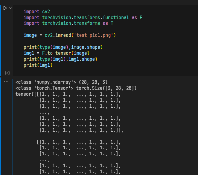
这里的to_tensor的大致实现如下:
def to_tensor(pic):
    """Convert a ``PIL Image`` or ``numpy.ndarray`` to tensor.
    This function does not support torchscript.

    See :class:`~torchvision.transforms.ToTensor` for more details.

    Args:
        pic (PIL Image or numpy.ndarray): Image to be converted to tensor.

    Returns:
        Tensor: Converted image.
    """
    if not(F_pil._is_pil_image(pic) or _is_numpy(pic)):
        raise TypeError('pic should be PIL Image or ndarray. Got {}'.format(type(pic)))

    if _is_numpy(pic) and not _is_numpy_image(pic):
        raise ValueError('pic should be 2/3 dimensional. Got {} dimensions.'.format(pic.ndim))

    default_float_dtype = torch.get_default_dtype()


    if isinstance(pic, np.ndarray):
        # handle numpy array
        # 如果是灰度的二维图像,加一个通道维度
        if pic.ndim == 2:
            pic = pic[:, :, None]

        img = torch.from_numpy(pic.transpose((2, 0, 1))).contiguous()
        # backward compatibility
        # 除以255
        if isinstance(img, torch.ByteTensor):
            return img.to(dtype=default_float_dtype).div(255)
        else:
            return img

    if accimage is not None and isinstance(pic, accimage.Image):
        nppic = np.zeros([pic.channels, pic.height, pic.width], dtype=default_float_dtype)
        pic.copyto(nppic)
        return torch.from_numpy(nppic)

    # 处理PIL的照片
    if pic.mode == 'I':
        img = torch.from_numpy(np.array(pic, np.int32, copy=False))
    elif pic.mode == 'I;16':
        img = torch.from_numpy(np.array(pic, np.int16, copy=False))
    elif pic.mode == 'F':
        img = torch.from_numpy(np.array(pic, np.float32, copy=False))
    elif pic.mode == '1':
        img = 255 * torch.from_numpy(np.array(pic, np.uint8, copy=False))
    else:
        img = torch.ByteTensor(torch.ByteStorage.from_buffer(pic.tobytes()))

    img = img.view(pic.size[1], pic.size[0], len(pic.getbands()))
    # 把HCW转成CHW格式
    img = img.permute((2, 0, 1)).contiguous()
    if isinstance(img, torch.ByteTensor):
        return img.to(dtype=default_float_dtype).div(255)
    else: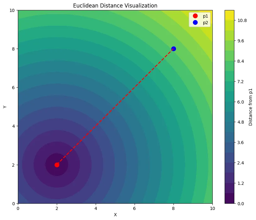
return img从熟悉的欧氏距离开始,一个经典的欧氏距离就是两点之间计算,公式如下:
d(p,q) = \sqrt {(p_1 - q_1 )^2 + (p_2 - q_2 )^2 }
在几何距离和数学建模常见的聚类(例如K-Means)计算相对常用。
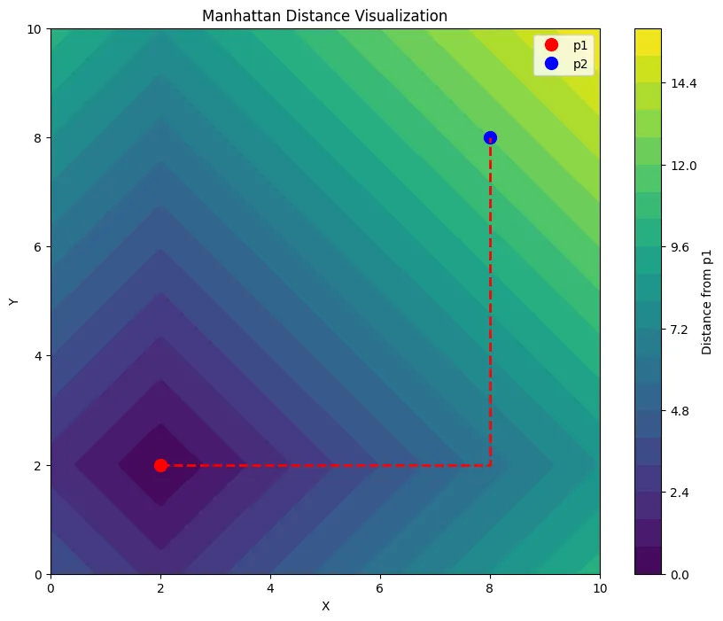
对于两个点之间的差异,还有一个常用于网格路径优化的距离就是曼哈顿距离,本身的定义是两个坐标在坐标轴上的绝对值之和。
d = \left| {x_1 - x_2 } \right| + \left| {y_1 - y_2 } \right|
pytorch的快速实现:
import torch
def EuclideanDistances(a,b):
    sq_a = a**2
    sum_sq_a = torch.sum(sq_a,dim=1).unsqueeze(1)  # m->[m, 1]
    print(sum_sq_a)
    sq_b = b**2
    sum_sq_b = torch.sum(sq_b,dim=1).unsqueeze(0)  # n->[1, n]
    bt = b.t()
    return torch.sqrt(sum_sq_a+sum_sq_b-2*a.mm(bt))
eu_dis = EuclideanDistances(img1.view(1,-1), img1.view(1,-1))
print(eu_dis) #两个tensor的欧氏距离,应该是0,但由于精度问题,结果会有误差,如果改为float64结果就稳定很多此时就得引入范数的概念了,因为pytorch使用的是统一的距离计算函数,采用的就是范数的概念。
对于一个n维的向量x = (x_1 ,x_2 ,x_3 ,{\rm{\cdot\cdot\cdot}},x_n ),p范数是向量各元素取p次方求和再开p次方根来衡量向量的长度。对应的式子:||x||_p = ( \sum_{i=1}^{n} |x_i|^p )^{1/p}
从这里也能看的出来,曼哈顿距离对应的就是L1的范数,欧氏距离对应的是L2范数,torch在CPU相关的代码如下,这里可以发现torch在传给具体硬件进行计算之前会将两个tensor进行广播和展平,在后续的运算中提供了数据的并行性。
template <typename F>
// 这里的张量是已经处理好的,
static void run_parallel_pdist(Tensor& result, const Tensor& self, const scalar_t p) {
  const scalar_t * const self_start = self.const_data_ptr<scalar_t>();
  const scalar_t * const self_end = self_start + self.numel();
  int64_t n = self.size(0);
  int64_t m = self.size(1);

  scalar_t * const res_start = result.data_ptr<scalar_t>();
  int64_t combs = result.numel(); // n * (n - 1) / 2

  // 并行计算,将输出索引k范围[0,comb-1]分成多个块,每个线程处理一段连续的k值
  parallel_for(0, combs, internal::GRAIN_SIZE / (16 * m), [p, self_start, self_end, n, m, res_start](int64_t k, int64_t end) {
    const Vec pvec(p);
    double n2 = n - .5;
    // The -1 accounts for floating point truncation issues
    // NOLINTNEXTLINE(bugprone-narrowing-conversions,cppcoreguidelines-narrowing-conversions)
    // 将k映射到矩阵的i和j
    int64_t i = static_cast<int64_t>((n2 - std::sqrt(n2 * n2 - 2 * k - 1)));
    int64_t j = k - n * i + i * (i + 1) / 2 + i + 1;

    const scalar_t * self_i = self_start + i * m;
    const scalar_t * self_j = self_start + j * m;
    scalar_t * res = res_start + k;
    const scalar_t * const res_end = res_start + end;

    while (res != res_end) {
      // 这里的向量化操作调用了CPU的SIMD,先计算|a-b|^p,再开p次方
      *res = F::finish(vec::map2_reduce_all<scalar_t>(
        [&pvec](Vec a, Vec b) { return F::map((a - b).abs(), pvec); },
        F::red, self_i, self_j, m), p);

      res += 1;
      self_j += m;
      if (self_j == self_end) {
        self_i += m;
        self_j = self_i + m;
      }
    }
  });
}在cuda的实现如下:
template <typename scalar_t, typename F>
__global__ static void cdist_backward_kernel_cuda_impl(scalar_t * buffer, const scalar_t * grad, const scalar_t * x1, const scalar_t * x2, const scalar_t * dist,
const scalar_t p, const int64_t r1, const int64_t r2, const int64_t m, const int64_t count, const int64_t r_size, const int64_t l1_size, const int64_t l2_size) {
// 线程分配
const int y = (blockIdx.y * gridDim.z + blockIdx.z) * blockDim.y + threadIdx.y;
const int init = blockIdx.x * blockDim.x + threadIdx.x;
if (y >= count || init >= m) {
return;
}
const int l = y / r_size;
const int k = y % r_size;
const int stride = blockDim.x * gridDim.x;
const int l_size = r_size * m;
int64_t i = k / r2;
int64_t j = k % r2;
const scalar_t grad_k = grad[y];
const scalar_t dist_k = dist[y];
const scalar_t * const start = x1 + l * l1_size + i * m;
const scalar_t * const end = start + m;
const scalar_t * self_i = start + init;
const scalar_t * self_j = x2 + l * l2_size + j * m + init;
scalar_t * buff_i = buffer + l * l_size + (r1 * j + i) * m + init;
// 内存访问连续
for (; self_i < end; self_i += stride, self_j += stride, buff_i += stride) {
const scalar_t res = F::backward(*self_i - *self_j, grad_k, dist_k, p);
*buff_i = res;
}
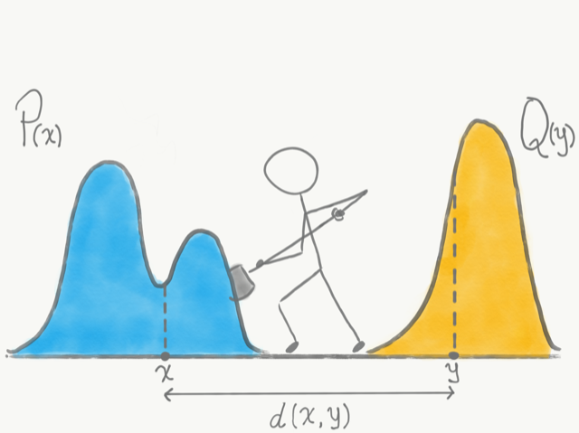
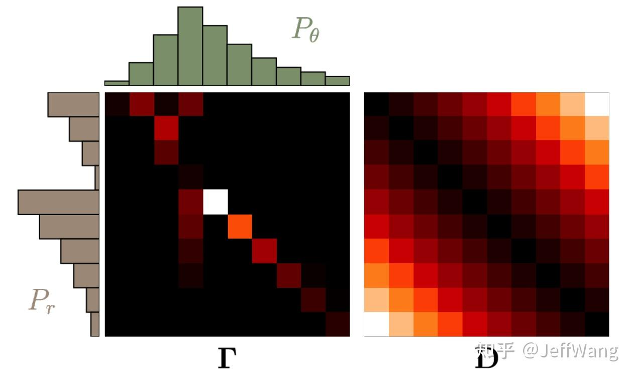
}在分布比较和一些GAN生成对抗网络(https://arxiv.org/abs/1701.07875)中,度量距离的方法有一个是Wasserstein距离的方法,这里的距离度量的就不是两个向量了,而是两个概率分布。我们将两个分布P,Q看成两堆土,如下图所示,希望把其中的一堆土移成另一堆土的位置和形状,有很多种可能的方案。推土代价被定义为移动土的量乘以土移动的距离,在所有的方案中,存在一种推土代价最小的方案,这个代价就称为两个分布的 Wasserstein 距离,也因此被称为推土机距离。
数学的表达太过复杂,不过有大佬写好了这些方便理解。
https://zhuanlan.zhihu.com/p/441197063
文章通过做功的方式给出了直观的理解,将求解处理成了线性规划问题。
先看一下每对图像之间的距离如何计算(调库)的:
query_image = cv2.imread('query_image.png', cv2.IMREAD_GRAYSCALE)
img = cv2.imread(f'image_{i}.png', cv2.IMREAD_GRAYSCALE)
hist, _ = np.histogram(query_image, bins=10, range=(0, 255), density=True)

# 计算距离,这里的cv2.DIST_L2正是之前提到的欧氏距离,在这里用来度量向量每个元素距离的
hist2, _ = np.histogram(img, bins=10, range=(0, 255), density=True)
distance = cv2.EMD(hist, hist2, cv2.DIST_L2)对应的代码文件是opencv源码仓库下的opencv/modules/imgproc/src/emd_new.cpp中,可以看到EMD函数本身是创建了个求解器进行计算的。
float cv::EMD(InputArray _sign1,
              InputArray _sign2,
              int distType,
              InputArray _cost,
              float* lowerBound,
              OutputArray _flow)
{
    CV_INSTRUMENT_REGION();

    Mat sign1 = _sign1.getMat();
    Mat sign2 = _sign2.getMat();
    Mat cost = _cost.getMat();

    CV_CheckEQ(sign1.cols, sign2.cols, "Signatures must have equal number of columns");
    CV_CheckEQ(sign1.type(), CV_32FC1, "The sign1 must be 32FC1");
    CV_CheckEQ(sign2.type(), CV_32FC1, "The sign2 must be 32FC1");

    const int dims = sign1.cols - 1;
    const int size1 = sign1.rows;
    const int size2 = sign2.rows;

    Mat flow;
    if (_flow.needed())
    {
        _flow.create(sign1.rows, sign2.rows, CV_32F);
        flow = _flow.getMat();
        flow = Scalar::all(0);
        CV_CheckEQ(flow.type(), CV_32FC1, "Flow matrix must have type 32FC1");
        CV_CheckTrue(flow.rows == size1 && flow.cols == size2,
                     "Flow matrix size does not match signatures");
    }

    DistFunc dfunc = 0;
    if (distType == DIST_USER)
    {
        if (!cost.empty())
        {
            CV_CheckEQ(cost.type(), CV_32FC1, "Cost matrix must have type 32FC1");
            CV_CheckTrue(cost.rows == size1 && cost.cols == size2,
                         "Cost matrix size does not match signatures");
            CV_CheckTrue(lowerBound == NULL,
                         "Lower boundary can not be calculated if the cost matrix is used");
        }
        else
        {
            CV_CheckTrue(dfunc == NULL, "Dist function must be set if cost matrix is empty");
        }
    }
    else
    {
        CV_CheckNE(dims, 0, "Number of dimensions can be 0 only if a user-defined metric is used");
        switch (distType)
        {
            case cv::DIST_L1: dfunc = distL1; break;
            case cv::DIST_L2: dfunc = distL2; break;
            case cv::DIST_C: dfunc = distC; break;
            default: CV_Error(cv::Error::StsBadFlag, "Bad or unsupported metric type");
        }
    }

    EMDSolver state;
    const bool result = state.init(sign1, sign2, dims, dfunc, cost, lowerBound);
    if (!result && lowerBound)
    {
        return *lowerBound;
    }
    // 调用迭代求解的函数
    state.solve();
    return (float)(state.calcFlow(_flow.needed() ? &flow : 0) / state.getWeight());
}

// 开始迭代求解
void EMDSolver::solve()
{
    if (ssize > 1 && dsize > 1)
    {
        const float eps = CV_EMD_EPS * max_cost;
        for (int itr = 1; itr < MAX_ITERATIONS; itr++)
        {
            /* find basic variables */
            if (findBasicVars() < 0)
                break;

            /* check for optimality */
            const float min_delta = checkOptimal();

            if (min_delta == CV_EMD_INF)
                CV_Error(cv::Error::StsNoConv, "");

            /* if no negative deltamin, we found the optimal solution */
            if (min_delta >= -eps)
                break;

            /* improve solution */
            if (!checkNewSolution())
                CV_Error(cv::Error::StsNoConv, "");
        }
    }
}求解的基本集中于findBasicVars这块,对应的代码在下面,可以看到opencv是通过将u和v的节点做成一个链表进行管理,数据上并没有并行,从计算本身也没看出什么并行。
int EMDSolver::findBasicVars() const
{
    int i, j;
    int u_cfound, v_cfound;
    Node1D u0_head, u1_head, *cur_u, *prev_u;
    Node1D v0_head, v1_head, *cur_v, *prev_v;
    bool found;

    CV_Assert(u != 0 && v != 0);

    /* initialize the rows list (u) and the columns list (v) */
    u0_head.next = u;
    for (i = 0; i < ssize; i++)
    {
        u[i].next = u + i + 1;
    }
    u[ssize - 1].next = 0;
    u1_head.next = 0;

    v0_head.next = ssize > 1 ? v + 1 : 0;
    for (i = 1; i < dsize; i++)
    {
        v[i].next = v + i + 1;
    }
    v[dsize - 1].next = 0;
    v1_head.next = 0;

    /* there are ssize+dsize variables but only ssize+dsize-1 independent equations,
       so set v[0]=0 */
    v[0].val = 0;
    v1_head.next = v;
    v1_head.next->next = 0;

    /* loop until all variables are found */
    u_cfound = v_cfound = 0;
    while (u_cfound < ssize || v_cfound < dsize)
    {
        found = false;
        if (v_cfound < dsize)
        {
            /* loop over all marked columns */
            prev_v = &v1_head;
            cur_v = v1_head.next;
            found = found || (cur_v != 0);
            for (; cur_v != 0; cur_v = cur_v->next)
            {
                float cur_v_val = cur_v->val;

                j = (int)(cur_v - v);
                /* find the variables in column j */
                prev_u = &u0_head;
                for (cur_u = u0_head.next; cur_u != 0;)
                {
                    i = (int)(cur_u - u);
                    if (getIsX(i, j))
                    {
                        /* compute u[i] */
                        cur_u->val = getCost(i, j) - cur_v_val;
                        /* ...and add it to the marked list */
                        prev_u->next = cur_u->next;
                        cur_u->next = u1_head.next;
                        u1_head.next = cur_u;
                        cur_u = prev_u->next;
                    }
                    else
                    {
                        prev_u = cur_u;
                        cur_u = cur_u->next;
                    }
                }
                prev_v->next = cur_v->next;
                v_cfound++;
            }
        }

        if (u_cfound < ssize)
        {
            /* loop over all marked rows */
            prev_u = &u1_head;
            cur_u = u1_head.next;
            found = found || (cur_u != 0);
            for (; cur_u != 0; cur_u = cur_u->next)
            {
                float cur_u_val = cur_u->val;
                i = (int)(cur_u - u);
                /* find the variables in rows i */
                prev_v = &v0_head;
                for (cur_v = v0_head.next; cur_v != 0;)
                {
                    j = (int)(cur_v - v);
                    if (getIsX(i, j))
                    {
                        /* compute v[j] */
                        cur_v->val = getCost(i, j) - cur_u_val;
                        /* ...and add it to the marked list */
                        prev_v->next = cur_v->next;
                        cur_v->next = v1_head.next;
                        v1_head.next = cur_v;
                        cur_v = prev_v->next;
                    }
                    else
                    {
                        prev_v = cur_v;
                        cur_v = cur_v->next;
                    }
                }
                prev_u->next = cur_u->next;
                u_cfound++;
            }
        }

        if (!found)
            return -1;
    }

    return 0;
}

文章评论